WILL Part I: Relational Geometry & R.O.M.

Interactive page — highlight any text to ask WILL AI for an explanation.

What is this page?

Welcome. This is the friendly entrance to WILL Relational Geometry — Part I, together with its companion Relational Orbital Mechanics (R.O.M.). They are one continuous derivation, not two separate papers.

The idea is simple to state: begin from a single principle — spacetime ≡ energy — and let geometry do the rest. From that one move, with zero free parameters, you recover Special and General Relativity, the Minkowski and Schwarzschild intervals, the equivalence principle, and the entire algebra of orbital motion.

This page is the accessible walk-through. The complete, line-by-line rigour lives in the papers, and every step here links to the exact section that proves it — so you can read for the story and dive for the proof whenever you like.

This is part of the WILL Trilogy: Part I — Relational Geometry (this page, with R.O.M.); Part II — Relational Cosmology; Part III — Relational Quantum Mechanics.

For the full papers and reproducible notebooks → Documents & Results
For quantitative, falsifiable predictions → Predictions
For questions and curiosity → Ask WILL AI

WILL: Relational Geometry — constructing reality from one principle

Instead of describing observed phenomena with externally added laws, this model generates the laws of physics as necessary consequences of its single principle — the shift from descriptive physics (write laws that fit observation) to generative physics (show why nothing else is possible).

Stage 0 — The Last Geocentric Epicycle

Every standard theory — SR, GR, QFT, the Standard Model, ΛCDM — is written with a two-part syntax: a fixed structure (a manifold plus a metric) plus the dynamics (fields and constants) that play out upon it. No observation demands this duplication; it is kept only because the resulting Lagrangians work inside the split. So the split is not an empirical discovery — it is an unjustified ontological commitment.

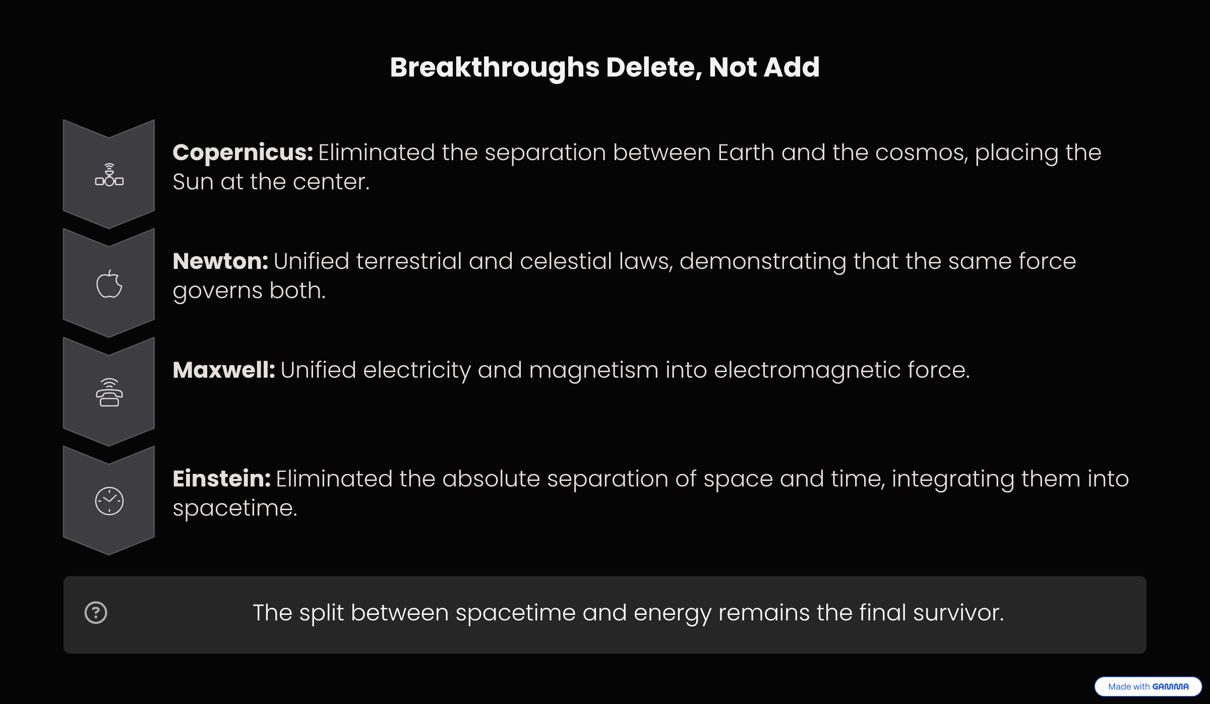
Breakthroughs in physics delete a false separation rather than adding entities

History keeps making the same move: it removes a false separation rather than adding entities. Copernicus deleted the Earth/cosmos divide; Newton, the terrestrial/celestial split; Maxwell, electricity/magnetism; Einstein, space/time. Each step widened the relational circle and reduced the number of unexplained primitives. The spacetime–energy split is the one survivor of that pruning.

The spacetime–energy split is the last geocentric epicycle in physics.

Full text: WILL RG Part I — Stage 0: The Last Geocentric Epicycle.

Stage I — Ontological Construction: The Primitives

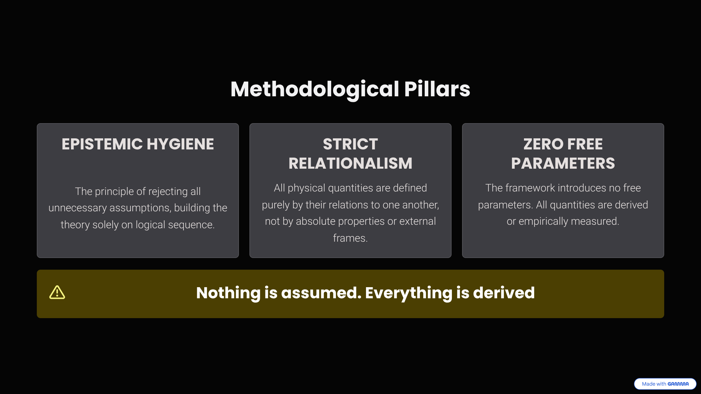
The four methodological principles

The framework rests on four methodological principles. They are not claims about reality but rules of epistemic purity; everything that follows is forced by them. “Zero free parameters” is a consequence of these principles, not a separate pillar.

Epistemic Hygiene — derive physics by removing hidden assumptions, never by introducing new postulates. No construct is kept unless geometrically or energetically necessary.
Relational Origin — every physical quantity is defined exclusively by its relations. Any absolute property reintroduces a metaphysical artefact.
Ontological Minimalism — keep the minimum number of primitives. Absolute background — container, time axis, absolute distance, forces, fields — is excluded as a primitive.
Mathematical Transparency — every symbol maps to exactly one physical idea. Number of symbols = number of independent physical ideas.

Full text and the derivation flow chart: Part I — Foundational Methodological Principles · Logos Map.

Energy as a conserved, relational, causal measure of change

Three results about the foundational core follow immediately from the four principles. They are the load-bearing theorems of everything below.

Theorem — Relational Closure

A purely relational system cannot be geometrically open. Any interaction with a supposed “outside” is itself a relation, and the moment it acts it is integrated into the system. An interacting non-relation is a contradiction; the system is closed by analytic necessity, not by a boundary.

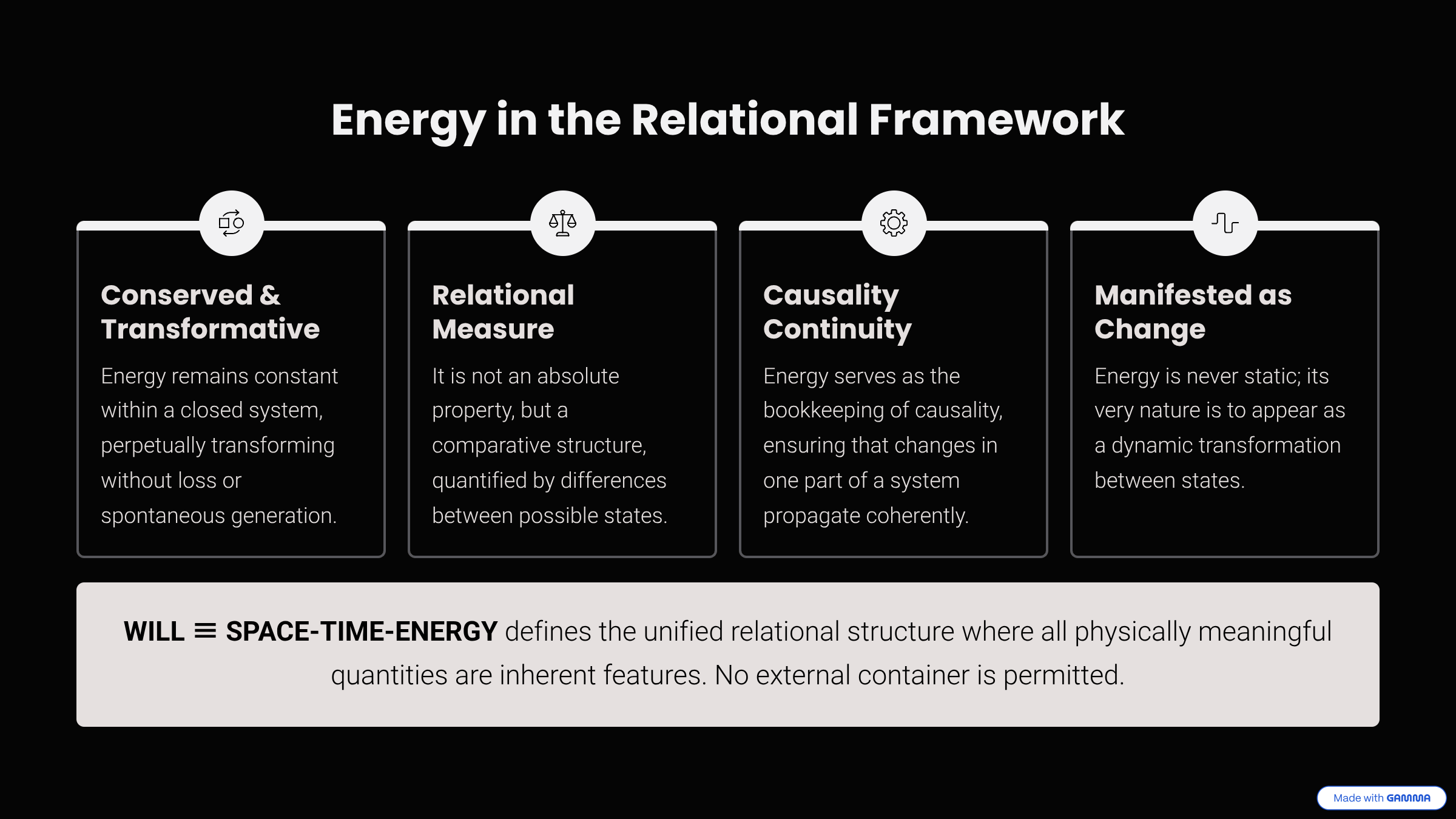
Theorem — Relational Invariance (the definition of Energy)

Within a closed system in which change occurs, every change must be balanced by a complementary change elsewhere. There must therefore exist a conserved measure of change. That invariant is what is historically called energy; proving it geometrically strips it of any substance and reveals it as the bookkeeping of causality.

Energy is the invariant relational measure of state transformation within a relationally closed system.

Theorem — Relational Isotropy

With no background grid, no direction can be privileged a priori; assigning an intrinsic axis to the unmeasured resource is unobservable surplus ontology. The carrier of the conserved resource must therefore be maximally symmetric.

Full text: Part I — The Foundational Core: Relational Geometry.

The Unifying Principle

Treating “structure” as separate from “dynamics” smuggles in a background container no phenomenon requires. Removing that separation forces structure and dynamics to be two aspects of one entity — a principle with negative ontological weight: it subtracts a primitive rather than adding one.

SPACETIME ≡ ENERGY

The single unified relational structure is named WILL ≡ SPACE–TIME–ENERGY; every physically meaningful quantity is a relational feature of WILL. The principle is foundational but testable: it must survive a geometric audit (its internal logical consequences) and an empirical audit (agreement with data). The remainder of this page is that audit — and the count of primitives drops from two (a container and its content) to one (a single self-relating structure).

Full text: Part I — Unifying Ontological Principle.

Stage II — Geometric Derivation

The two minimal carriers

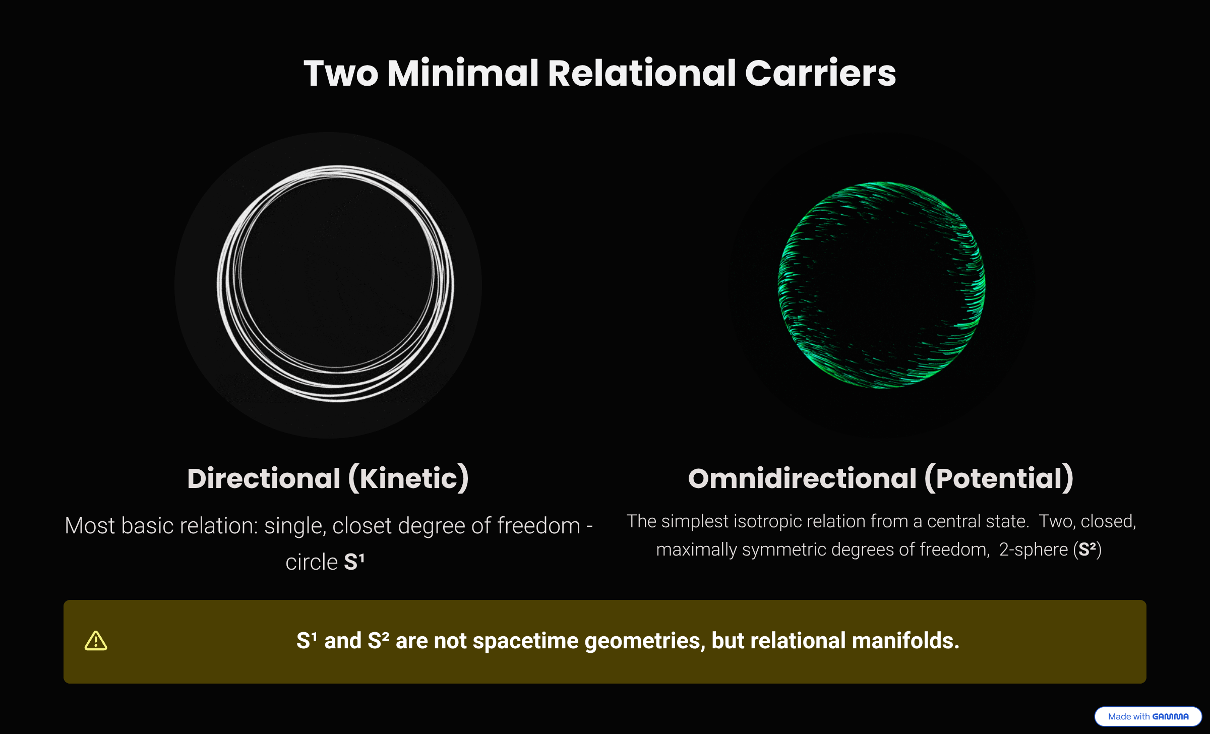
The circle S¹ for directional relations and the sphere S² for omnidirectional relations

Closure, Conservation and Isotropy fix the only carriers the conserved resource can use. A directional relation (one degree of freedom) that cannot leak must close into a loop, and the unique parameter-free, maximally symmetric loop is the circle \(S^1\). An omnidirectional relation (two degrees of freedom) that is closed and isotropic can only be the sphere \(S^2\). No free integers, no preferred axes.

A note on what \(S^1\) and \(S^2\) are. They are not shapes embedded in space. \(S^2\) has no physical surface area, no volume, and does not “dilute” a flux across a distance. They are abstract relational carriers encoding closure, conservation and isotropy. Spatial distance \(r\) and time are descriptive labels attached to these patterns — the projection dictates the space, not the reverse.

Full text: Part I — Deriving Relational Carriers.

Amplitude, phase, and the Conservation of Relation

The β projection on the S¹ unit circle

By the Relational Origin Principle, the identification of spacetime with energy needs two complementary measures: an amplitude (external shift) and a phase (internal order). Any description of change must be of relational origin — a single number introduces an absolute value, which the Relational Origin Principle forbids. The carriers \(S^1\) and \(S^2\) supply the minimal geometry that enforces this: their orthogonal projections give exactly two non-redundant, coupled axes.

Amplitude (\(\beta\), \(\kappa\)) — the external shift from the observer’s rest frame. On \(S^1\), \(\beta\) is what we measure as relative speed, \(\beta = v/c\); on \(S^2\), \(\kappa\) measures gravitational depth, \(\kappa = v_e/c\).
Phase (\(\beta_Y\), \(\kappa_X\)) — the internal ordering: proper time and proper length. Phase \(=1\) is rest; phase \(=0\) is the light-speed / horizon limit.

Theorem — Conservation of Relation

For both kinematic (\(S^1\)) and potential (\(S^2\)) modes, the sum of the squared Amplitude and squared Phase is strictly invariant:

\[\text{Amplitude}^2 + \text{Phase}^2 = 1\]

Proof. The conserved relational resource is carried by the maximally symmetric geometries \(S^1\) and \(S^2\). Normalizing the total conserved resource to unity, any physical state corresponds to a point on these carriers. The algebraic identity of orthogonal projections on a unit circle and sphere dictates that the sum of their squares equals the squared radius. Therefore \(\beta^2 + \beta_Y^2 = 1\) and \(\kappa^2 + \kappa_X^2 = 1\), encoding the finite, closed relational budget.

The projections are cross-cultural invariants

\(S^1\) is the minimal structure that can encode a directional relation without absolute space. Its parameter is an angle \(\theta_1\) whose cosine \((\beta = \cos\theta_1)\) we identify with the fraction \(v/c\), and whose sine \((\beta_Y = \sin\theta_1)\) governs the internal ordering (proper-time fraction).

\(S^2\) is the minimal structure that can encode an omnidirectional relation without absolute space. Its parameter is an angle \(\theta_2\) whose sine \((\kappa = \sin\theta_2)\) we identify with the escape-velocity fraction \(v_e/c\), and whose cosine \((\kappa_X = \cos\theta_2)\) governs the internal ordering.

Any two observers assign \(\beta\) and \(\kappa\) the same value for the same state, whatever their unit system — or even their descriptive vocabulary:

\[\beta = \frac{v}{c}, \qquad \kappa = \frac{v_e}{c} = \sqrt{\frac{R_s}{r}} = \sqrt{\frac{\rho}{\rho_{max}}}\]

are translations into descriptive vocabulary.

These two facts — that \(\beta\) and \(\kappa\) are pinned to closed carriers, and that they read out identically for every observer — are what make them behave like measured invariants rather than adjustable labels. You read \(\kappa\) straight off a spectrum as gravitational redshift, \(\kappa^2 = 1 - 1/(1+z_\kappa)^2\), with no mass and no \(G\) in sight. From this single constraint everything downstream is forced: the energy–momentum relation, the Minkowski and Schwarzschild intervals, the equivalence principle, and the entire orbital algebra below.

Full text: Part I — The Amplitude–Phase Duality & Conservation of Relation.

Where spatial distance comes from (the inverse-square law)

Spatial distance is derived as the operational inverse of relational phase capacity. Treating distance as an a priori primitive would violate Relational Origin and Ontological Minimalism.

Theorem — Inverse-Square

The inverse-square potential proportionality \(\kappa^2 \propto 1/r\) is a geometric necessity of the \(S^2\) carrier’s relational capacity, determined without spatial primitives.

Proof. By the Spectroscopic Phase Shift Theorem, the potential projection \(\kappa^2\) is extracted entirely from the dimensionless phase tension \(z_\kappa\), independent of spatial parameters. Distance must therefore be defined by the relational tension between energy states. Normalizing the absolute geometric scale at saturation \((\kappa^2 = 1 \equiv r = R_s)\), distance \(r\) emerges as the reciprocal measure of the omnidirectional projection amplitude:

\[\kappa = \sin\theta_2 \;\Longrightarrow\; \kappa^2 = \frac{R_s}{r} \;\Longrightarrow\; r = \frac{R_s}{\kappa^2} \;\Longrightarrow\; \kappa^2 \propto 1/r.\]

The \(1/r\) proportionality is an analytic identity defining spatial distance, not an empirical input.

The inverse-square law does not exist because physical space dictates how forces dilute. It exists because “spatial distance” is the descriptive vocabulary assigned to the inverse capacity of the omnidirectional relational carrier \(S^2\).

Full text: Part I — Relational Origin of the Inverse-Square Law and the Nature of Spatial Distance.

Consequence: relativistic effects

Proposition — Relativistic effects

The conservation law implies that any redistribution between the orthogonal components manifests physically as the relativistic effects of time dilation and length contraction.

Proof. By Conservation of Relation, \(\beta^2 + \beta_Y^2 = 1\) and \(\kappa^2 + \kappa_X^2 = 1\). An increase in Amplitude \((\beta, \kappa)\) enforces a geometric decrease in Phase \((\beta_Y, \kappa_X)\). This reduction of \(\beta_Y\) and \(\kappa_X\) corresponds precisely to the dilation of proper time and the contraction of proper length, while the growth of \(\beta\) and \(\kappa\) represents momentum or potential depth. The trade-off is the direct, un-parameterized expression of the geometric closure of the carriers.

This identifies relativistic and gravitational time dilation not as a mysterious “slowing down” of clocks, but as geometric phase rotation. As a system invests more of its relational existence into external Amplitude, it necessarily withdraws from its internal Phase, changing the rate of its proper-time evolution.

The geometry of spacetime is dictated by the relations of energy states.

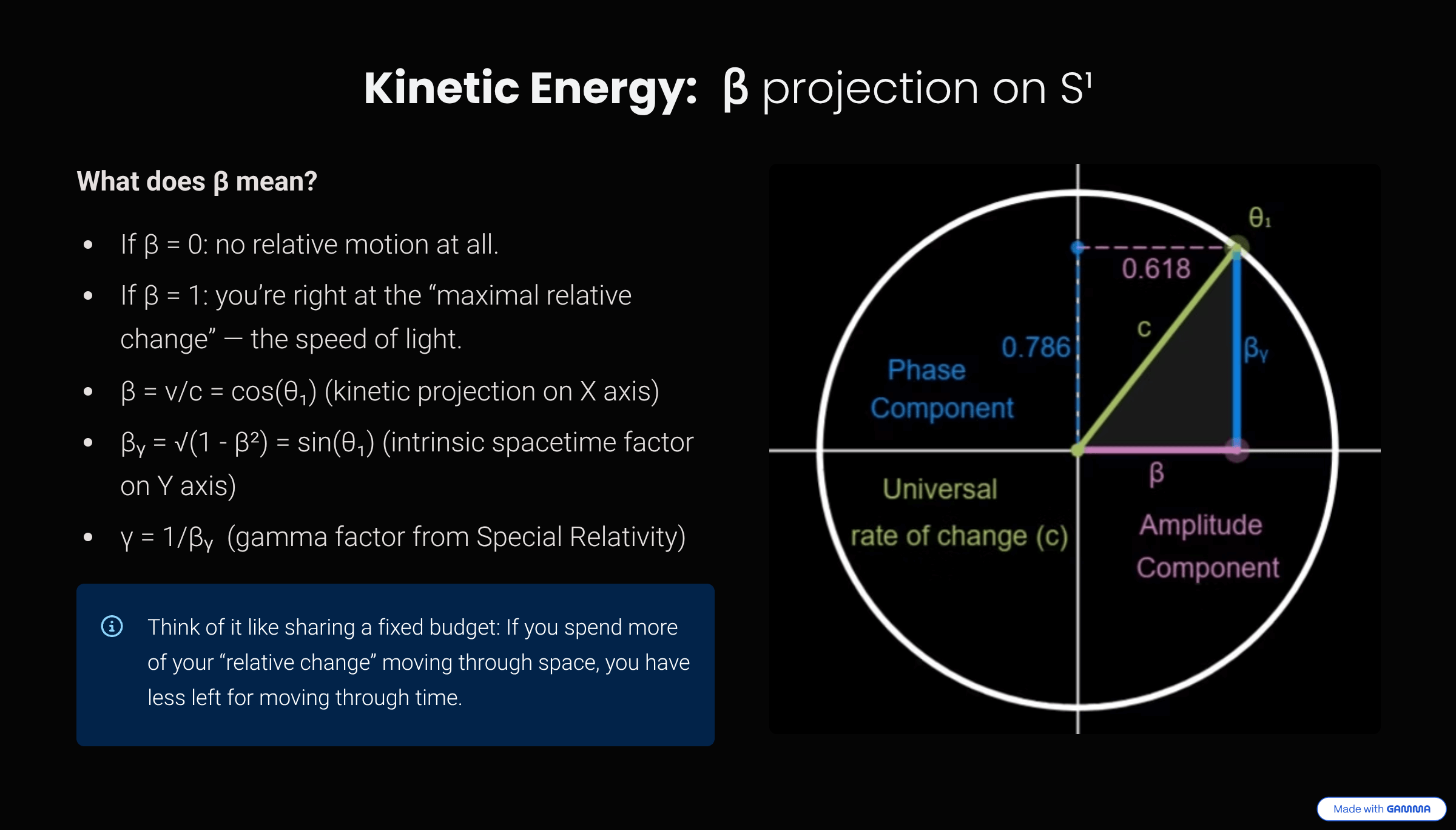
Kinetic energy on \(S^1\): rest energy, mass, momentum

Energy–momentum identity on the S¹ circle

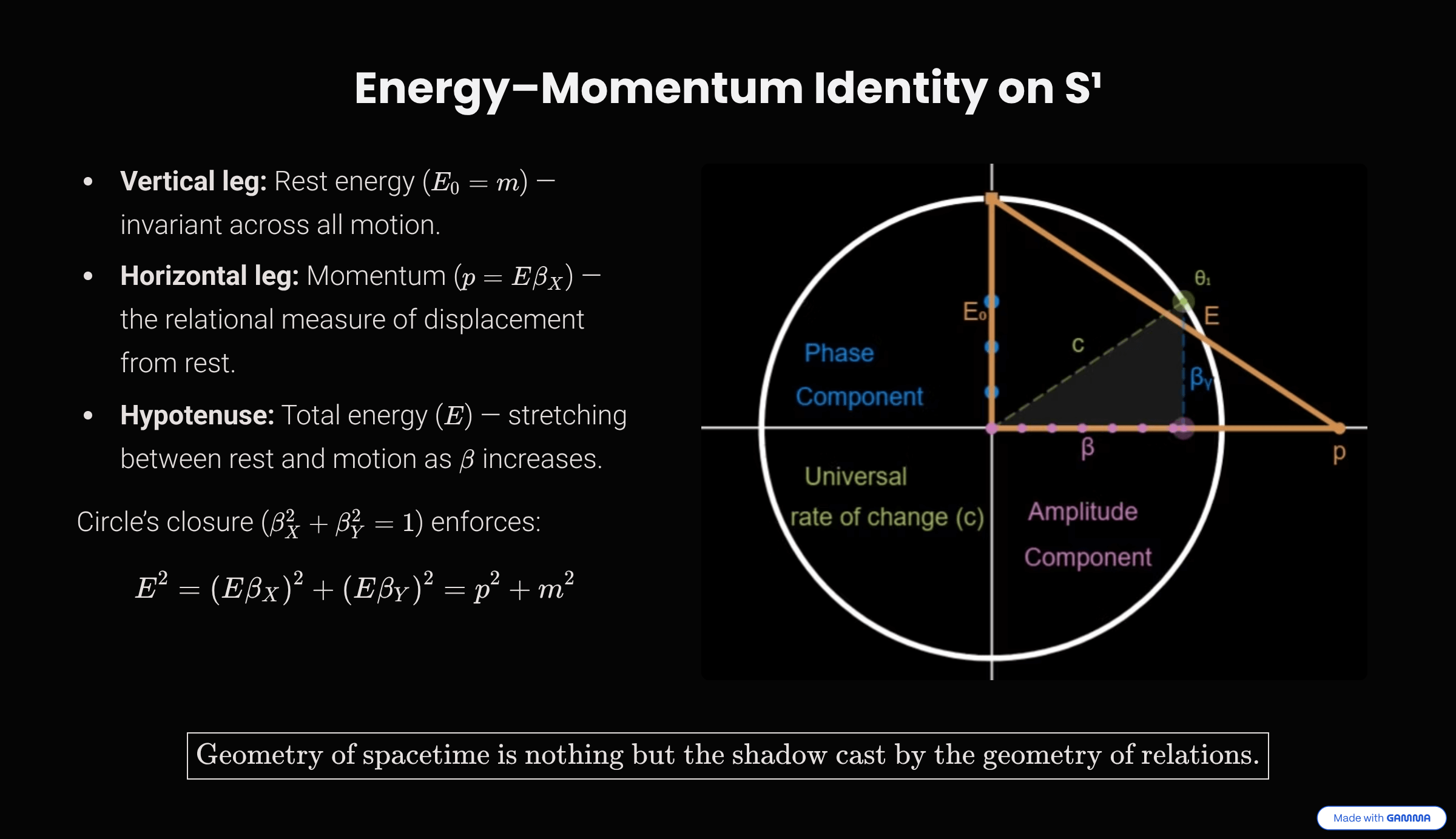
Total energy projects onto both axes, \(E_X = E\beta\) and \(E_Y = E\beta_Y\). The vertical projection turns out to be invariant.

Theorem — Invariant Projection of Rest Energy

For any state \((\beta, \beta_Y)\) on the circle \(S^1\), the total energy \(E\) scales so that its vertical projection stays constant and equal to the rest energy \(E_0\): \(\;E\beta_Y = E_0.\)

Proof. By the Relational Origin Principle and the Conservation Theorem, a system’s internal energy measured in its own rest frame \((\beta = 0 \implies \beta_Y = 1)\) is its rest energy, \(E_0\). For another frame \(B\) observing system \(A\), if \(A\) is in relative motion \((\beta > 0)\), the total energy \(E\) differs, but the internal energy \(E_Y\) must remain an invariant property of \(A\). To preserve this invariant and agree on measurements, frame \(B\) must measure \(A\)’s internal phase projection as identical to the rest energy:

\[E_{Y_{B \leftarrow A}} = E_{Y_{A \leftarrow A}} = E_0.\]

Therefore the internal energy \(E_Y\) measured externally by any frame remains constant and equal to the rest energy, \(E_Y \equiv E_0\), where \(E_0\) is the energy measured in the frame where the system is at rest. Geometric consistency then fixes the vertical leg:

\(E_Y = E\beta_Y = E_0 \implies E = \frac{E_0}{\beta_Y}.\)

The historical Lorentz factor is just the reciprocal of the phase, \(\gamma = 1/\beta_Y\). Within \(c = 1\) the invariant rest energy is the mass, \(E_0 = m\): the identities \(E_0 = mc^2\) and \(m = E_0/c^2\) reduce to tautologies, so mass is not independent but the rest-energy invariant itself. Identifying momentum with the horizontal projection \(p \equiv E\beta\), closure gives the standard relation as a pure geometric identity of \(S^1\):

\(E^2 = p^2 + m^2 \quad\Longrightarrow\quad E^2 = (pc)^2 + (mc^2)^2\)

Full text: Part I — Kinetic Energy Projection β on S¹.

The Minkowski interval is the inflated form of \(S^1\) closure

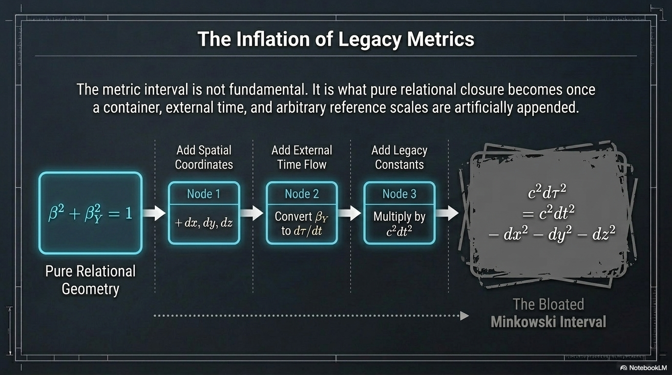
Minkowski interval as the inflation of S¹ closure

In textbook Special Relativity the Minkowski interval is the starting point. WILL reverses the order: the primitive is the dimensionless closure \(\beta^2 + \beta_Y^2 = 1\), which contains no coordinates, no container, no external time. The interval is what that relation becomes once four substantival posits are added — a container; spatial coordinates \(x, y, z\); an externally flowing time \(t\) (demoting the phase to \(\beta_Y \equiv d\tau/dt\)); and a reference scale \(c^2 dt^2\). Substituting \(\beta^2 = (dx^2+dy^2+dz^2)/(c^2 dt^2)\) and \(\beta_Y = d\tau/dt\) into closure returns the interval exactly:

\(c^2 d\tau^2 = c^2 dt^2 - dx^2 - dy^2 - dz^2\)

The interval carries more structure than the relation it encodes. The relation is primary; the metric is its inflation.

Full text: Part I — Minkowski Interval as Inflation of the S¹ Closure.

Gravity: the potential projection \(\kappa\) on \(S^2\)

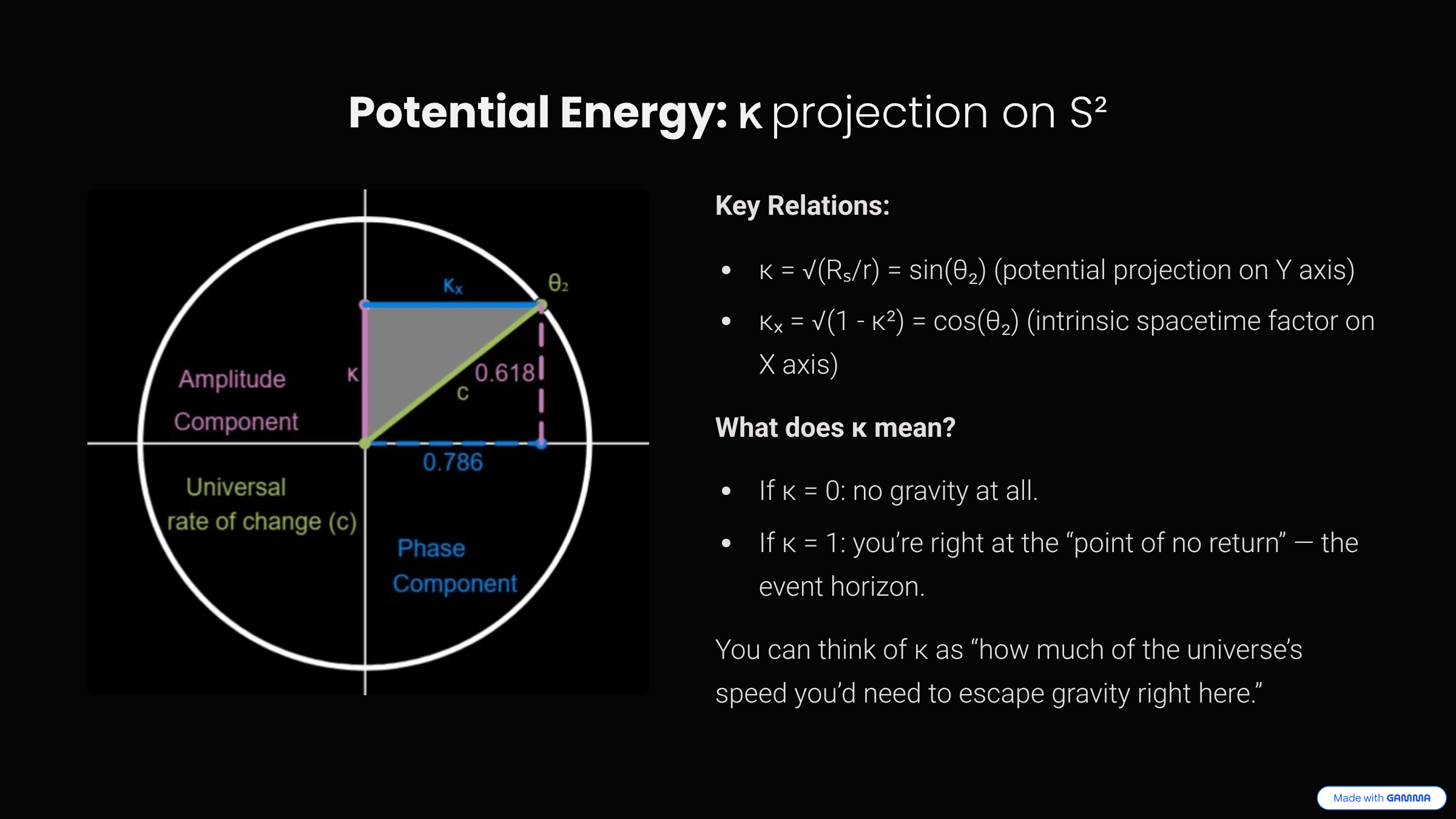
The κ projection on the S² unit sphere

Everything above repeats on the sphere. The amplitude \(\kappa = v_e/c = \sqrt{R_s/r}\) measures gravitational depth (\(\kappa = 1\) is the horizon, \(r = R_s\)), the phase \(\kappa_X\) governs gravitational time and length, and \(\kappa^2 + \kappa_X^2 = 1\). The same trade-off — more amplitude \(\kappa\), less phase \(\kappa_X\) — is what we observe as gravitational time dilation. Curved spacetime is the shadow cast by this conserved relation.

The Schwarzschild interval is the inflated form of \(S^2\) closure

Strictly parallel. Start from \(\kappa^2 + \kappa_X^2 = 1\). Append a container around a central body, hold the observer static, posit an externally flowing time so \(\kappa_X \equiv d\tau/dt\), and localize the amplitude as \(\kappa^2 \equiv R_s/r\) — which is what first introduces the radial coordinate \(r\) and the legacy constants \(G, M\) via \(R_s = 2GM/c^2\). Closure then yields the Schwarzschild time component exactly:

\(c^2 d\tau^2 = c^2\left(1 - \frac{R_s}{r}\right) dt^2\)

Here \(\kappa\) is the primitive; \(r\), \(G\) and \(M\) are coordinate-and-unit artifacts attached to it. R.O.M. (below) describes gravitating systems fully without \(G\) and \(M\), confirming the projection — not \(R_s/r\) — is irreducible. The full Schwarzschild and Kerr line elements are recovered in R.O.M.

Full text: Part I — Schwarzschild Interval as Inflation of the S² Closure · R.O.M. — Schwarzschild Metric.

Closure: the relational origin of the virial theorem

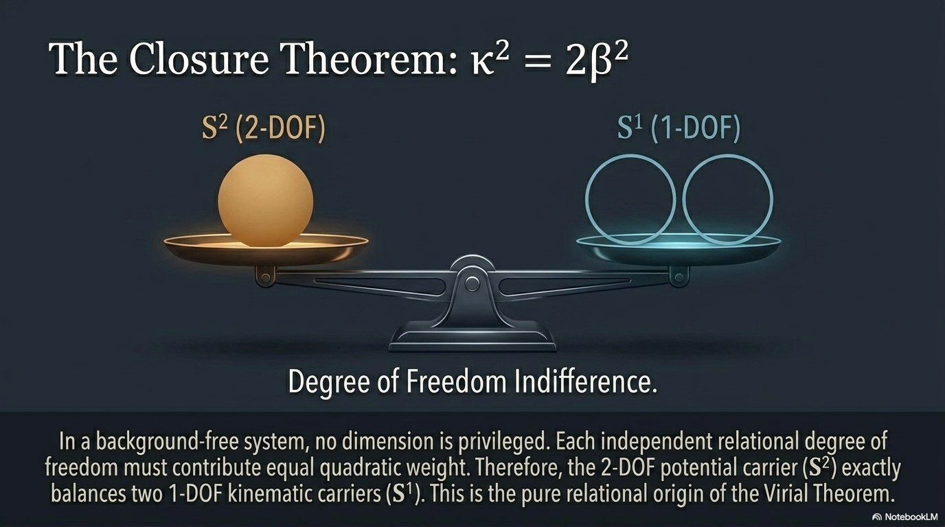
The exchange rate κ²=2β² from the ratio of degrees of freedom

The exchange rate between the potential and kinematic projections of a closed system is the ratio of the carriers’ degrees of freedom. Under maximal symmetry and ontological minimalism, each independent degree of freedom carries equal quadratic weight; \(S^2\) has two degrees of freedom and \(S^1\) has one, so the rate is \(2\):

\(\kappa^2 = 2\beta^2\)

This is the relational origin of the virial theorem, and it fixes the carrier saturations: \(S^1\) at \(\beta^2 = 1\) (light), \(S^2\) at \(\kappa^2 = 2\) (the extremal-Kerr state). It also serves as a diagnostic, through the closure factor \(\delta \equiv \kappa^2/2\beta^2\): for circular orbits \(\delta = 1\); for elliptical orbits \(\delta\) breathes around the cycle but averages to \(1\); for a radiating binary \(\delta \neq 1\), the defect measuring exactly the energy carried off by gravitational waves.

Potential distribution (\(\kappa^2\)) ≡ 2 × kinetic distribution (\(\beta^2\)).

Full text: Part I — Closure: Relational Origin of the Virial Theorem.

The Total Relational Shift \(Q\)

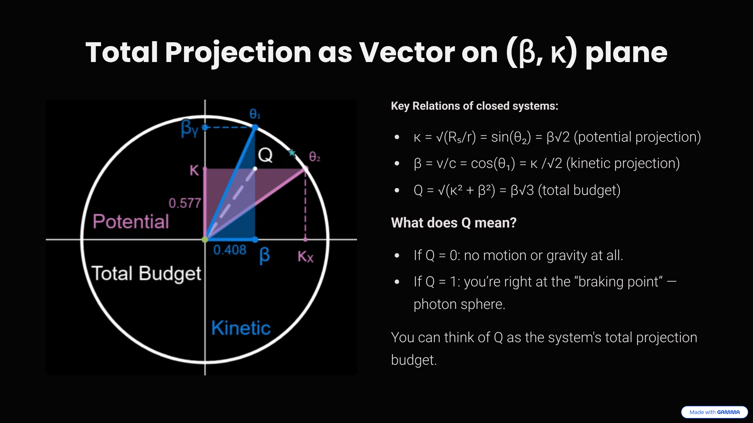
The total relational shift Q on the β–κ plane

When an observer targets another system, the combined kinematic and gravitational state difference is one magnitude — the norm \(Q\), not a direction:

\(Q^2 = \beta^2 + \kappa^2 \qquad (\text{closed systems: } Q^2 = 3\beta^2)\)

\(Q\) is genuinely relational: each observer sits at their own origin \((\beta, \kappa) = (0, 0)\) (self-centering), so both parties assign the same magnitude to each other, \(Q_{A \to B} = Q_{B \to A}\). There is no shared background arena — only mutual shift magnitudes computed from each origin. Causal interaction requires the other system’s centre to lie within one’s horizon, \(Q < 1\); at \(Q = 1\) the budget is exhausted (the photon-sphere / null-circumnavigation limit).

Full text: Part I — Total Relational Shift Q · Relational Reciprocity.

The Energy-Symmetry Law

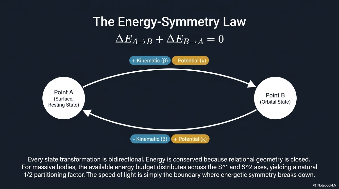
Every transformation is bidirectional: a change observed by \(A\) corresponds to an equal and opposite change observed by \(B\). This is causal continuity in algebraic form.

Theorem — Energy Symmetry

The specific energy differences (per unit rest energy) for a transition between two states balance to zero:

\(\Delta E_{A \to B} + \Delta E_{B \to A} = 0.\)

Two consequences follow. The speed limit \(v \le c\) is built in: if \(\beta > 1\), the kinetic budget and the required transfer grow without bound, no finite reverse transfer could balance it, and the symmetry would break — so \(\beta \le 1\) is a requirement of causal consistency, not a separate postulate. Light is the single-axis limit: for light \(\beta = 1 \Rightarrow \beta_Y = 0\), the internal phase vanishes, there is no rest frame, and the whole resource sits on one axis. This removes the \(\tfrac12\) partitioning, so the gravitational effect on light is exactly twice that on a massive body (\(\Phi_\gamma = \kappa^2 c^2\) vs \(\Phi_{\text{mass}} = \tfrac12\kappa^2 c^2\)) — the observed factor of 2 in light deflection and the Shapiro delay, with no weak-field expansion.

Causality is a built-in feature of Relational Geometry.

Full text: Part I — Energy-Symmetry Law · Single-Axis Transfer and the Nature of Light.

Stage III — Legacy Translation: recovering the known machinery

Before testing anything against data, watch the familiar tools of physics reappear as special cases of the relations above.

The equivalence principle as a derived identity

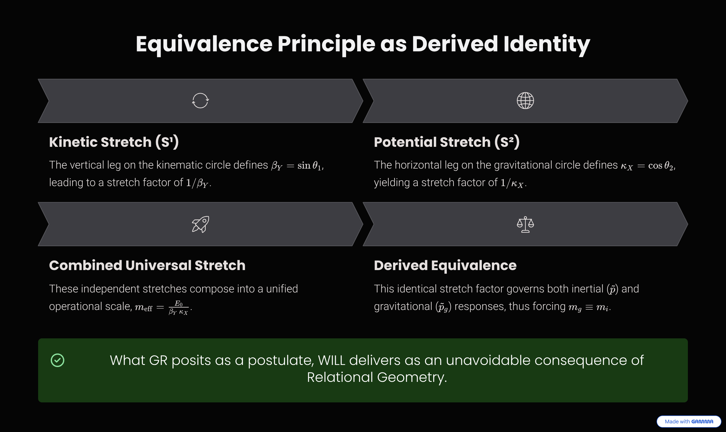
In General Relativity \(m_g \equiv m_i\) is an independent postulate. In WILL it is forced. Both projections rescale the same invariant \(E_0\), so composing the two stretches gives one local energy scale:

\[E_{\text{loc}} = \frac{E_0}{\beta_Y\,\kappa_X} = \frac{E_0}{\sqrt{(1-\beta^2)(1-\kappa^2)}} = \frac{E_0}{\tau}\]

The inertial and gravitational responses share one effective mass \(m_{\text{eff}} = E_0/(\tau c^2)\); every internal energy channel scales by the same \(1/\tau\), so the ratios cancel in every observable — which is composition-independent free fall (Eötvös universality). Hence \(m_g \equiv m_i \equiv m_{\text{eff}}\): what GR posits, WILL delivers as a corollary.

Full text: Part I — Equivalence Principle as Derived Identity.

Classical mechanics as collapses of the two-point law

Four ontological collapses of the two-point law

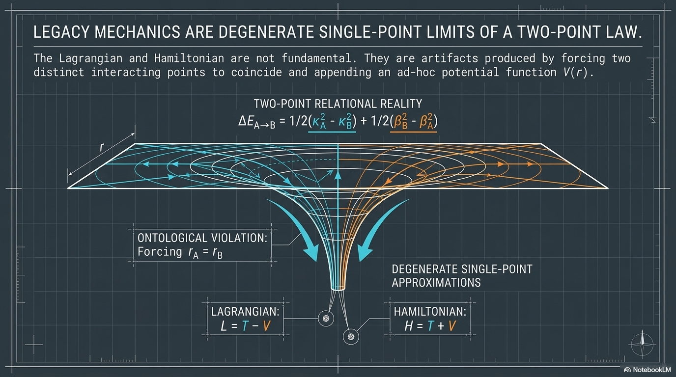
The two-point Energy-Symmetry Law is more fundamental than the standard tools of mechanics. Each appears when the two-point relation \(A \leftrightarrow B\) is collapsed onto a single point — forcing \(r_A = r_B = r\) and then re-introducing, by hand, the structure the collapse discarded.

The Lagrangian, Hamiltonian, Newton’s third law and the Einstein–Hilbert action are single-point shadows of one two-point law.

Full text: Part I — Two-Point Origin of the Lagrangian and Hamiltonian.

Relational Orbital Mechanics (R.O.M.)

Relational Orbital Mechanics

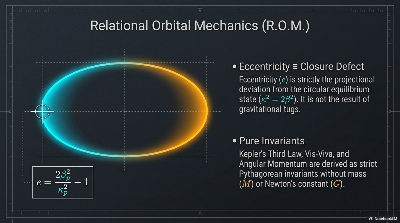
R.O.M. is not a separate paper — it is the operational payoff of the same principles applied to bound gravitating systems. It is a closed algebraic system that classifies the allowed relational states of an orbit with no differential equations, no acceleration term, no \(G\) and no \(M\). Everything below derives from \(\beta\), \(\kappa\) and closure \(\kappa^2 = 2\beta^2\).

Full paper: R.O.M. — Relational Orbital Mechanics · interactive: R.O.M. Desmos.

R.O.M. does not describe how a body moves under forces; it classifies the algebraically allowed relational states of a bound system. The whole system is generated from two operational inputs — the gravitational redshift \(z_\kappa\) and the transverse Doppler shift \(z_\beta\) — together with the closure law. The core registry:

\[\kappa^2 = 1 - \frac{1}{(1+z_\kappa)^2}, \qquad \beta^2 = 1 - \frac{1}{(1+z_\beta)^2}\] \[\tau = \kappa_X\,\beta_Y = \frac{1}{(1+z_\kappa)(1+z_\beta)}, \qquad Q^2 = \kappa^2 + \beta^2, \qquad \kappa^2 = 2\beta^2\] \[R_s = \frac{Tc}{\pi}\beta^3, \qquad a = \frac{R_s}{\kappa^2}, \qquad \rho = \frac{\kappa^2 c^2}{8\pi G a^2}, \qquad \Delta\varphi = \frac{2\pi\,\tau_Y^2}{1-e^2}, \qquad e = \frac{1}{\delta_p} - 1\]

Each line is an identity among dimensionless projections; \(G\) and \(M\) appear only at the very end, as unit-conversion factors, never as inputs.

Full registry: R.O.M. — Closed Algebraical System of R.O.M. Equations.

Relational origin of the orbital laws

Each classical orbital law reappears as a strict algebraic identity of the relational projections — no force, no acceleration primitive, no background metric.

Spectroscopic shifts — \(\kappa\) and \(\beta\) are observables. By the Conservation Theorem and self-centering, \(\kappa^2 = 1 - 1/(1+z_\kappa)^2\) and \(\beta^2 = 1 - 1/(1+z_\beta)^2\): the projections are extracted directly from measured gravitational redshift and transverse Doppler shift, independent of \(G\) and \(M\). The single optical observable \(\tau\) carries the complete structural state, \(\tau^2 = 1 - Q^2 + \kappa^2\beta^2\). (R.O.M. — Spectroscopic Shifts)

Kepler’s Third Law. From \(\beta = 2\pi a/cT\) and \(\kappa^2 = R_s/a\), closure \(\kappa^2 = 2\beta^2\) gives directly \(a^3 = \frac{R_s c^2}{8\pi^2}\,T^2\), i.e. \(a \propto T^{2/3}\) — with no mass and no gravitational constant. (R.O.M. — Kepler’s Third Law)

Eccentricity ≡ closure defect. Eccentricity is the projectional deviation from circular equilibrium \(\delta = 1\): \(\;e = \frac{1}{\delta_p} - 1 = \frac{2\beta_p^2}{\kappa_p^2} - 1 = 1 - \frac{2\beta_a^2}{\kappa_a^2}\), derived from the conservation of the relational projections without forces. (R.O.M. — Eccentricity)

Vis-viva as a Pythagorean identity. The Newtonian \(v^2/2 - GM/r = -GM/2a\) becomes a strict orthogonal sum on the carriers: the local potential projection is the Pythagorean square sum of the radial, transverse and global kinetic projections, \(\kappa_o^2(o) = \beta_R^2(o) + \beta_T^2(o) + \beta^2\), with the global binding invariant \(\kappa_o^2(o) - \beta_o^2(o) = \beta^2\) constant at every orbital phase. (R.O.M. — Vis-Viva)

Classical acceleration and angular momentum. The radial gradient of the orbital invariant \(\kappa_o^2 - \beta_o^2 = \beta^2\), with \(\kappa_o^2 = R_s/r\), yields \(a_{acc} = -\frac{R_s c^2}{2r^2} = -\frac{GM}{r^2}\) — Newton’s law, with no force primitive. The transverse-projection invariant gives a phase-independent specific angular momentum \(h = R_s c\,\frac{\sqrt{1-e^2}}{2\beta}\). (R.O.M. — Acceleration · Angular Momentum)

Orbital precession as phase accumulation. Precession is the exact algebraic accumulation of the internal phase divergence over a closed cycle — no perturbation series, no truncation:

\[\Delta\varphi = \frac{2\pi\,\tau_Y^2}{1-e^2}, \qquad \tau_Y^2 \equiv 1 - \tau^2 = Q^2 - \kappa^2\beta^2\]

The cross-coupling \(\kappa^2\beta^2\) is the non-linear interaction between the \(S^1\) and \(S^2\) carriers — the exact term GR’s first-order formula omits. (R.O.M. — Orbital Precession as Phase Accumulation)

Dynamic event horizon. At total saturation \(\kappa^2 = 1\) (so \(\beta^2 = \tfrac12\), \(\tau \to 0\), \(\tau_Y \to 1\)) a circular orbit precesses by \(\Delta\varphi = 2\pi\) per revolution: the periapsis shifts by a full circle, the trajectory folds onto itself, and forward motion nullifies itself. The horizon is the unitary topological closure of the relational trajectory — not a point of infinite density in a container. (R.O.M. — Dynamic Event Horizon)

Gravitational deflection and lensing (the factor of 2, exactly). The phase buffer \(\beta_Y\) sets the interaction gradient \(\Gamma(\beta) = \tfrac{1+\beta^2}{2}\): a slow body has a full buffer (\(\Gamma = \tfrac12\)); light exhausts it (\(\beta = 1 \Rightarrow \Gamma = 1\)), absorbing twice the gradient. This yields one exact, expansion-free deflection law for any trajectory, reducing to \(\Delta\gamma = 2\arcsin(\kappa_p^2/\kappa_{Xp}^2)\) for light and to an exact algebraic Einstein ring for lensing.

R.O.M. — Gravitational Deflection and Lensing

Time-density invariant and the absolute scale. The invariant \(\tau_D = T\sin(\theta)^{3/2} = \sqrt{\pi/G\rho}\) fixes the central density from period and angular radius alone, and at the horizon gives the universal constant \(\tau_{D(\rm limit)}/R_s = 2\sqrt{2}\,\pi/c\). Four independent algebraic routes (optical-phase, two-point differential, geometric-resonance, instantaneous) determine the absolute system scale \(R_s\) from observables, none of them passing through \(2GM/c^2\). (R.O.M. — Time-Density Invariant · Absolute Scale, Methods A–D)

Rotation: Kerr without a metric. Setting \(\beta = ac^2/GM\) and \(\kappa = \sqrt{2}\,\beta\), the relational carriers reproduce the Kerr structure algebraically: inner/outer horizons \(r_\pm = \tfrac{R_s}{2}(1 \pm \beta_Y)\), merging at the extremal limit \(\beta = 1\) to \(r_{\min} = \tfrac12 R_s\), the ergosphere \(r_{\rm ergo} = \tfrac{R_s}{2}(1 + \sqrt{1 - \beta^2\cos^2\theta})\), and a ring singularity. No naked singularity emerges for \(\beta \le 1\) — cosmic censorship is enforced directly by the Energy-Symmetry Law bounding \(\beta \in [0, 1]\). (R.O.M. — Kerr Without Metric)

Frame-dragging as a chiral algebraic asymmetry. What GR derives from the off-diagonal \(g_{t\phi}\) metric component, R.O.M. obtains from linear phase superposition on the directed \(S^1\) carrier: the composite \(\beta_\Sigma = \beta_{\rm orb} \pm \beta_{\rm spin}\) under closure produces the symmetry-breaking cross-term \(\pm 4\beta_{\rm orb}\beta_{\rm spin}\), mandating that prograde orbits sit deeper than retrograde. Ablating higher-order terms recovers the post-Newtonian Lense–Thirring node precession exactly; tested against LAGEOS-1 it agrees with observation and GR. (R.O.M. — Chiral Asymmetry / Frame-Dragging)

Density, the field equation, and no singularities

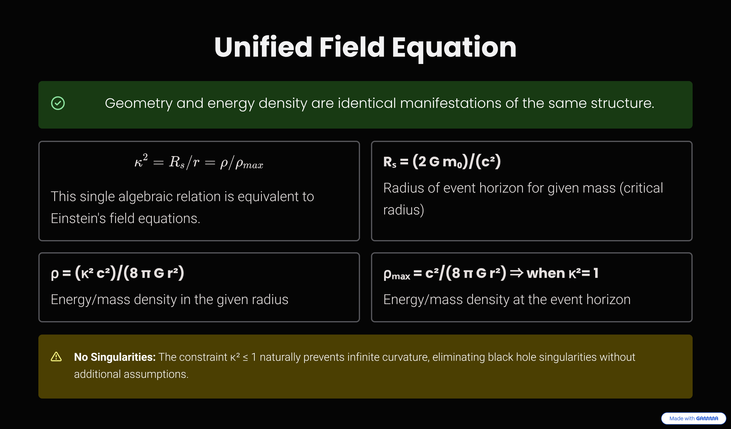
The unified geometric field equation

Normalizing the potential projection over the unit-sphere area gives the local energy density and its bound at saturation:

\[\rho = \frac{\kappa^2 c^2}{8\pi G r^2}, \qquad \rho_{\text{max}} = \frac{c^2}{8\pi G r^2}\]

so all of gravitational physics reduces to a single algebraic identity — the ratio of geometric scales equals the ratio of energy densities:

\(\kappa^2 = \frac{R_s}{r} = \frac{\rho}{\rho_{\text{max}}}\)

Because density is capped at a finite \(\rho_{\text{max}}\), infinite density is impossible. The static horizon sits at \(\kappa^2 = 1\) (\(r = R_s\)); even the extremal rotating limit only reaches \(r = R_s/2\). The point \(r = 0\) is simply absent from the admissible relational range — singularities are excluded by construction, not patched over.

Density is bounded; the point \(r = 0\) does not exist.

Full text: Part I — Density, Mass, and Pressure · No Singularities, No Hidden Regions.

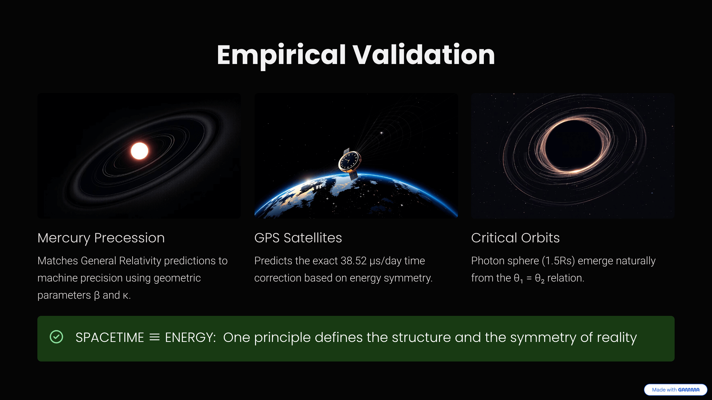
Empirical Alignment — the framework against reality

Everything to this point was geometry and logic. Now the same projections meet measured data. In several cases the standard formula turns out to be the first-order approximation of an exact relational expression.

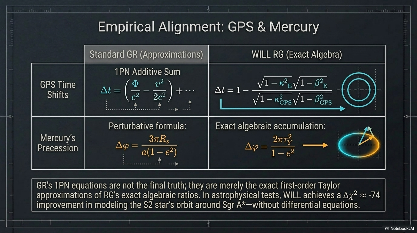
Earth–GPS: standard GR as the first-order approximation of RG

The daily clock offset between GPS satellites and the ground combines kinematic (SR) and gravitational (GR) effects into one relational factor \(\tau = \beta_Y\kappa_X\). RG composes them multiplicatively; the textbook formula adds them. The additive form is exactly the first-order Taylor coefficient of the RG ratio — proved symbolically and to 40-digit precision.

Full text and notebook: Part I — Earth–GPS System.

Reconstructing the Solar System from observations alone

Reconstructing absolute scale from four dimensionless observations

This is the centrepiece. Take four numbers any observer can measure — no rulers laid out in space, no mass, no gravitational constant — and rebuild the entire Mercury–Sun system: its absolute scale, its orbit, and its 43″/century precession. The inputs are pure ratios:

the Sun’s angular radius in the sky, \(\theta_\odot = 0.0046524\) rad
the Sun’s surface redshift, \(z_{\rm sun} = 2.1224\times10^{-6}\)
Mercury’s orbital-period ratio to Earth, \(T_M/T_\oplus = 0.2408\)
Mercury’s eccentricity, \(e_M = 0.2056\)

The chain is short enough to follow by hand:

Scale ratio: \(\;R_{ratio} = \dfrac{\theta_\odot}{(T_M/T_\oplus)^{2/3}\,(1 - e_M)} \approx 0.0151290\)
Potential at perihelion: \(\;\kappa_p^2 = \left[1 - \dfrac{1}{(1+z_{\rm sun})^2}\right] R_{ratio} \approx 6.4219\times10^{-8}\)
Kinetic at perihelion: \(\;\beta_p^2 = \dfrac{\kappa_p^2}{2}(1 + e_M) \approx 3.8712\times10^{-8}\)
Global invariants: \(\;\beta^2 = \kappa_p^2 - \beta_p^2 \approx 2.5508\times10^{-8}, \quad \kappa^2 = 2\beta^2\)
Precession: \(\;\Delta\varphi = \dfrac{2\pi\,\tau_Y^2}{1 - e_M^2} \approx 5.0203\times10^{-7}\ \text{rad/orbit} = \mathbf{43.015''/century}\)
Absolute scale: \(\;R_s = \dfrac{T_M\,c\,\beta^3}{\pi} \approx 2954.8\ \text{m}\) (GR: \(2GM_\odot/c^2 \approx 2953.33\) m — a \(0.05\%\) difference)
Orbit: \(\;a = \dfrac{R_s}{\kappa^2} \approx 5.792\times10^{10}\ \text{m}, \quad r_p = \dfrac{R_s}{\kappa_p^2} \approx 4.601\times10^{10}\ \text{m}\)

Every standard value of the Mercury–Sun system, recovered from four dimensionless observations. The same chain, with only Jupiter’s period ratio and eccentricity swapped in, rebuilds Jupiter’s orbit to \(0.038\%\) — so this is a universal property of bound systems, not a quirk of Mercury. \(G\) and \(M\) never enter except as the final unit conversion; \(R_s\) is the primary geometric invariant, and classical mass is the anthropocentric proxy for it.

You don’t need a PhD to follow this — it’s a handful of ratios and square roots. The best way to believe it is to do it yourself.

Reproduce it yourself → Interactive Desmos: rebuild the Solar System from ratios · Colab notebook

Full derivation: R.O.M. — Relational Parameterization and the Fundamental Primitives.

Mercury’s precession: GR 1PN as the first-order approximation of RG

Empirical validation of R.O.M.

Substituting closure and the field relation into the exact precession law gives a closed form whose first term is identically the standard post-Newtonian formula, with a single explicit correction:

\[\Delta\varphi_{\rm RG} = \underbrace{\frac{3\pi R_s}{a(1-e^2)}}_{\text{GR 1PN}} - \frac{\pi R_s^2}{a^2(1-e^2)}, \qquad \Delta\varphi_{\rm RG} - \Delta\varphi_{\rm GR} = -\frac{2\pi\,\beta^2\kappa^2}{1-e^2}\bigg|_{a}\]

The GR formula is recovered by a single explicit cancellation, \(\beta^2\kappa^2 \to 0\) in \(\tau_Y^2 = 1 - (1-\beta^2)(1-\kappa^2)\). This is an algebraic identity in \((R_s, a, e)\), verified symbolically and to 40-digit precision.

Full verification + notebook: R.O.M. — Mercury’s Precession: GR 1PN as First-Order Approximation of RG.

The S2 star at Sgr A*: R.O.M. against GR on real data

R.O.M. is confronted with the 24-year astrometric and radial-velocity dataset of the S2 star (174 raw observables), against two GR references — a time-linear 1PN pericentre advance and a direct numerical integration of the 1PN equations of motion — all carrying the same nine orbital parameters and zero free precession parameters.

The result, stated plainly: a bare nine-parameter fit favours R.O.M. by \(\Delta\chi^2 = 80.7\). But a reduced \(\chi^2 \approx 4.4\)–\(4.9\) rejects all three bare models — no published S2 analysis fits absolute sky positions without a reference-frame solution. When the standard linear calibration (frame zero-point, drift, instrument offsets) is granted identically to every model, the gap closes completely: \(\Delta\chi^2 = -0.5\) over 156 degrees of freedom. R.O.M. and General Relativity are statistically indistinguishable on the S2 orbit.

At current precision, R.O.M. is observationally equivalent to GR, reached from a closed dimensionless algebra (the advance magnitude matches GR 1PN to \(3\times10^{-5}\); the full scale follows from chronometric and spectroscopic ratios via \(R_s = Tc\beta^3/\pi\)). The genuine departure is of order \(\beta^4\), four orders of magnitude below S2 sensitivity. The falsifiable frontier is therefore not Galactic-Centre orbits but where \(\beta^4\) terms resolve: relativistic pulsar binaries, horizon-scale orbits, and gravitational-wave inspirals.

Full analysis + reproduction: R.O.M. — S2 Star (Sgr A*) Against General Relativity and Instrumental Systematics.

The three-body L1 point, from observations alone

The same algebraic chain locates the Sun–Earth L1 equilibrium point without \(G\), \(M\) or a metric. Enforcing closure and energy symmetry on the synchronous-motion condition yields an exact quintic in the normalised separation \(\alpha = (R_E - R_{L1})/R_E\), whose physical root reproduces the observed Earth–L1 distance \(R_{L1} \approx 1.5\times10^9\,\text{m}\) to better than \(0.3\%\). The chain that recovers Mercury’s precession and the S2 orbit also fixes a collinear three-body equilibrium.

Full derivation + notebook: R.O.M. — Relational Derivation of the L1 Equilibrium Point.

Stage IV — Consequences & Direct Applications

The Theoretical Ouroboros

The theoretical Ouroboros

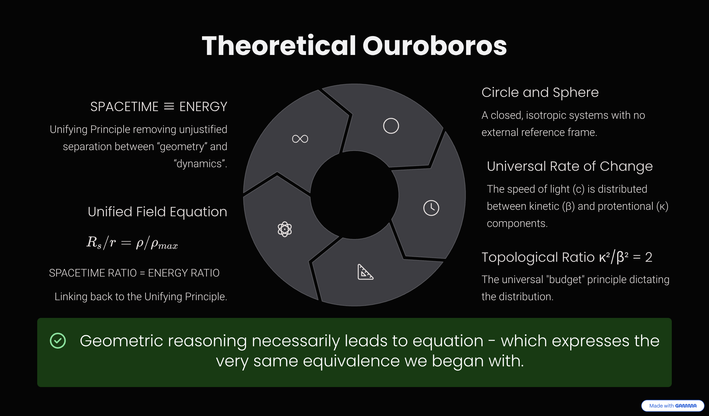
The single principle, through pure geometry, generated the carriers, the projections, and the laws — and those laws produced a field equation that states exactly the equivalence it began with: the ratio of geometric scales equals the ratio of energy densities.

SPACETIME ≡ ENERGY \(\;\Longrightarrow\;\) \(\kappa^2 = \dfrac{R_s}{r} = \dfrac{\rho}{\rho_{\text{max}}}\) \(\;\Longrightarrow\;\) SPACETIME ≡ ENERGY

The principle is proven as the inevitable consequence of its own geometric consistency. Beautiful as that is, the test stays empirical — which is why the section above meets data, not only logic.

Full text: Part I — Theoretical Ouroboros.

\(W_{ILL} = 1\) — the unity of the projections

The WILL invariant

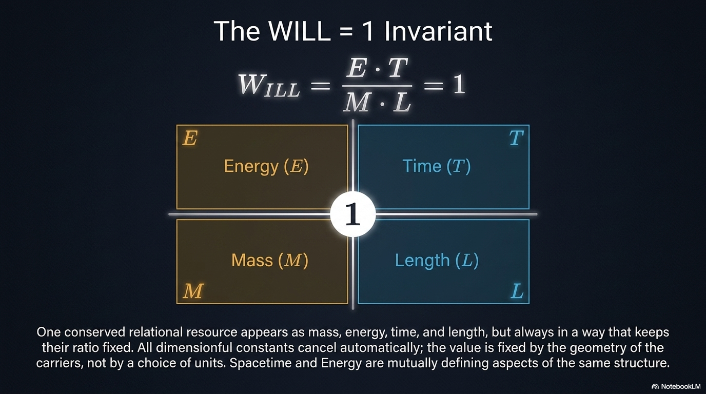
If there is one relational resource, then mass, energy, time and length are not independent — they are four correlated projections of the same structure. Combining them in the one dimensionless way the carriers permit gives an invariant identically equal to 1 for any closed system, at every energy, scale and orbital phase:

\(W_{ILL} = \frac{E\,T}{M\,L} = 1\)

All dimensionful constants cancel automatically; the value is fixed by the geometry of the carriers, not by a choice of units. Equivalently \(E/M = L/T\): the energy sector and the spacetime sector are locked together. Treating energy–mass and space–time as separate blocks is an interpretational approximation; \(W_{ILL} = 1\) is the precise statement that spacetime ≡ energy.

WILL is not the unit of something — but the Unity of Everything.

Full text: Part I — W_ILL: Unity of Relational Structure.

The name “WILL”

WILL stands for SPACE–TIME–ENERGY — both a shorthand and a quiet irony toward the anthropic principle. The universe is not a stage where energy acts through time upon space, but a single self-balancing structure whose internal distinctions generate every phenomenon. The cosmos does not possess “will”; yet through WILL it manifests all that is.

From descriptive to generative physics

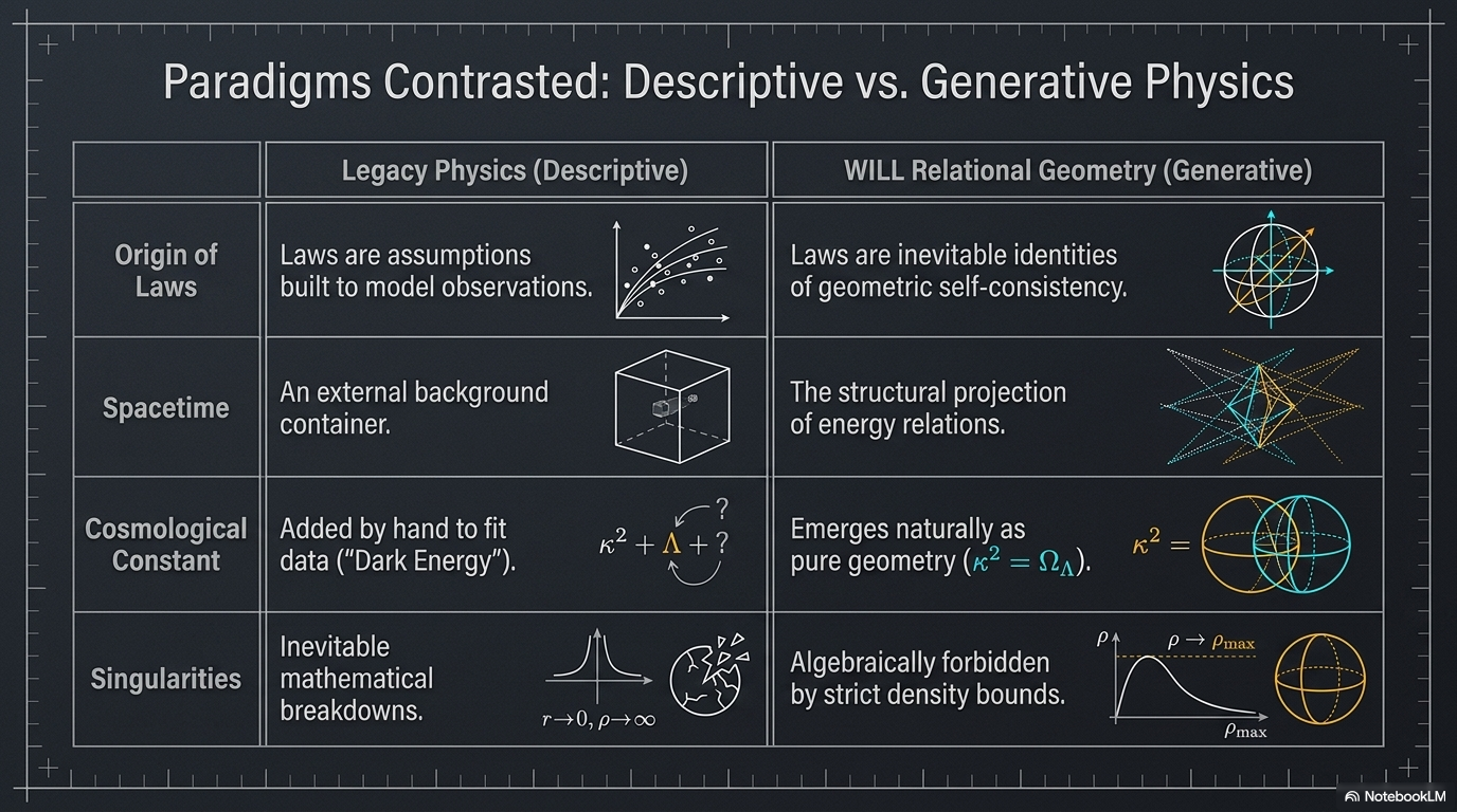
The deepest shift is not a new equation but a new role for physical law. Standard physics observes phenomena and then writes laws to describe them. WILL inverts this: the laws are generated as the only self-consistent possibility.

Descriptive physics (standard)	Generative physics (WILL)
Phenomena are observed, then summarized into empirical laws.	Laws emerge as inevitable consequences of relational geometry.
Physical laws are assumptions introduced to model reality.	Physical laws are identities enforced by geometric self-consistency.
Time and space are external backgrounds.	Time and space are projections of energy relations.
Dynamics = evolution of states in time.	Dynamics = ordered succession of balanced configurations; time is emergent.
Goal: describe what is observed.	Goal: show why nothing else is possible.

Full text: Part I — From Descriptive to Generative Physics.

Limitations and Challenges

This is open research, and the boundaries are stated plainly.

Current limitations. Gravitational waves and the full radiative two-body problem are not yet formulated relationally — only conservative, bound orbits are covered. A complete multi-body architecture beyond the collinear L1 case has not been constructed. These are limits of present mathematical facility rather than prohibitions of the ontology, and collaboration on radiative dynamics and multi-body closures is actively invited.

Falsifiability and future tests. The sharpest near-term discriminator is continued high-precision monitoring of the S2 star: RG predicts a true-anomaly-coupled precession phasing that should retain its statistical edge over the time-linear form as GRAVITY+ adds pericentre passages (2026–2028); a statistically significant reversal would count against the phasing hypothesis. The genuine point of departure is the \(\beta^4\) structure of the closure law, resolved only in relativistic pulsar binaries, horizon-scale orbits, and gravitational-wave inspirals.

Full text: Part I — Challenges and Current Limitations.

Conclusion

The entire phenomenology of motion — Keplerian architecture, perihelion precession, light deflection, frame-dragging, the L1 point — emerges as an algebraic consequence of the four methodological principles, an unbroken chain with zero flexibility. This is not a re-description of General Relativity; it is the irreducible algebraic core that remains when the ontological superstructure of Riemannian geometry and tensor formalism is removed. Within RG:

\(G\) and \(M\) are secondary. All scales follow from dimensionless spectroscopic and chronometric ratios; the gravitational constant and the kilogram appear only as unit conversions.
The metrics are derived. Minkowski, Schwarzschild and Kerr intervals are Pythagorean identities of the carriers \(S^1\) and \(S^2\), not postulates of a 4D manifold.
Closure replaces the virial theorem. \(\kappa^2 = 2\beta^2\) is the consequence of equal budget per degree of freedom.
Precession is topological, not dynamical. The pericentre advance is the mismatch of internal phase over one cyclic extension, with no geodesic integration.
Singularities are excluded. The point \(r = 0\) is absent from the admissible relational range.

Full text: WILL RG — Conclusion & the Trilogy.

This is Just a Beginning

This is Part I, with R.O.M. The same projections extend to cosmology (Part II) and quantum mechanics (Part III). The core remains: energy does not exist in spacetime — it creates spacetime by its projection.

Documents & Results · Testable Predictions · Ask WILL AI · Help This Research

💡 Select any text to ask WILL AI for an explanation.